import numpy as np
import scipy as sp
import matplotlib.pyplot as plt
import math as mt

plt.style.use("fivethirtyeight")
from statsmodels.graphics.tsaplots import plot_acf
Although we have demonstrated the convenience of PyMC3, which encapsulated the MCMC in the relatively isolated process, we still need to investigate the basic structure of MCMC.
In this chapter, we will demonstrate the inner mechanism of MCMC with the help of previous analytical examples. There will be no PyMC3 used in this Chapter.
Markov Chain Monte Carlo
The Markov Chain Monte Carlo (MCMC) is a class of algorithm to simulate a distribution that has no closed-form expression.
To illustrate the mechanism of MCMC, we resort to the example of Gamma-Poisson conjugate.
Though it has a closed-form expression of posterior, we can still simulate the posterior for demonstrative purpose.
To use MCMC, commonly the Bayes’ Theorem is modified without affecting the final result. \[ P(\lambda \mid y) \propto P(y \mid \lambda) P(\lambda) \] where \(\propto\) means proportional to, the integration in the denominator can be safely omitted since it is a constant.
Here we recap the example of hurricanes in the last chapter. The prior elicitation uses
\[ E(\lambda) = \frac{\alpha}{\beta}\\ \text{Var}(\lambda) = \frac{\alpha}{\beta^2} \]
x = np.linspace(0, 10, 100)
params = [10, 2]
gamma_pdf = sp.stats.gamma.pdf(x, a=params[0], scale=1 / params[1])

fig, ax = plt.subplots(figsize=(7, 7))
ax.plot(
    x, gamma_pdf, lw=3, label=r"$\alpha = %.1f, \beta =  %.1f$" % (params[0], params[1])
)
ax.set_title("Prior")
mean = params[0] / params[1]
mode = (params[0] - 1) / params[1]
ax.axvline(mean, color="tomato", ls="--", label="mean: {}".format(mean))
ax.axvline(mode, color="red", ls="--", label="mode: {}".format(mode))
ax.legend()
plt.show()
Because posterior will also be Gamma distribution, we start from proposing a value drawn from posterior \[ \lambda = 8 \] This is an arbitrary value, which is called the initial value.
Calculate the likelihood of observing \(k=3\) hurricanes given \(\lambda=8\). \[ \mathcal{L}(3 ; 8)=\frac{\lambda^{k} e^{-\lambda}}{k !}=\frac{8^{3} e^{-8}}{3 !}=0.1075 \]
def pois_lh(k, lamda):
    lh = lamda**k * np.exp(-lamda) / mt.factorial(k)
    return lh
lamda_init = 8
k = 3
pois_lh(k=k, lamda=lamda_init)0.02862614424768101- Calculate prior \[ g(\lambda ; \alpha, \beta)=\frac{\beta^{\alpha} \lambda^{\alpha-1} e^{-\beta \lambda}}{\Gamma(\alpha)} \]
def gamma_prior(alpha, beta, lamda):
    prior = (
        beta**alpha * lamda ** (alpha - 1) * np.exp(-beta * lamda)
    ) / sp.special.gamma(alpha)
    return prior
lamda_current = lamda_init
alpha = 10
beta = 2
gamma_prior(alpha=alpha, beta=beta, lamda=lamda_current)0.0426221247856141- Calculate the posterior with the first guess \(\lambda=8\) and we denote it as \(\lambda_{current}\)
k = 3
posterior_current = pois_lh(k=k, lamda=lamda_current) * gamma_prior(
    alpha=10, beta=2, lamda=lamda_current
)
posterior_current0.0012201070922556493- Draw a second value \(\lambda_{proposed}\) from a proposal distribution with \(\mu=\lambda_{current}\) and \(\sigma = .5\). The \(\sigma\) here is called tuning parameter, which will be clearer in following demonstrations.
tuning_param = 0.5
lamda_prop = sp.stats.norm(loc=lamda_current, scale=tuning_param).rvs()
lamda_prop6.903049306071834- Calculate posterior based on the \(\lambda_{proposed}\).
posterior_prop = gamma_prior(alpha, beta, lamda=lamda_prop) * pois_lh(
    k, lamda=lamda_prop
)
posterior_prop0.005584813985229831- Now we have two posteriors. To proceed, we need to make some rules to throw one away. Here we introduce the Metropolis Algorithm. The probability threshold for accepting \(\lambda_{proposed}\) is \[ P_{\text {accept }}=\min \left(\frac{P\left(\lambda_{\text {proposed }} \mid \text { data }\right)}{P\left(\lambda_{\text {current }} \mid \text { data }\right)}, 1\right) \]
print(posterior_current)
print(posterior_prop)
0.0012201070922556493
0.005584813985229831prob_threshold = np.min([posterior_prop / posterior_current, 1])
prob_threshold1.0It means the probability of accepting \(\lambda_{proposed}\) is \(1\). What if the smaller value is \(\frac{\text{posterior proposed}}{\text{posterior current}}\), let’s say \(\text{prob_threshold}=.768\). The algorithm requires a draw from a uniform distribution, if the draw is smaller than \(.768\), go for \(\lambda_{proposed}\) if larger then stay with \(\lambda_{current}\).
- The demonstrative algorithm will be
if sp.stats.uniform.rvs() > 0.768:
    print("stay with current lambda")
else:
    print("accept next lambda")
accept next lambda- If we accept \(\lambda_{proposed}\), redenote it as \(\lambda_{current}\), then repeat from step \(2\) for thousands of times.
Combine All Steps
We will join all the steps in a loop for thousands of times (the number of repetition depends on your time constraint and your computer’s capacity).
def gamma_poisson_mcmc(
    lamda_init=2, k=3, alpha=10, beta=2, tuning_param=1, chain_size=10000
):
    np.random.seed(123)
    lamda_current = lamda_init

    lamda_mcmc = []
    pass_rate = []
    post_ratio_list = []

    for i in range(chain_size):
        lh_current = pois_lh(k=k, lamda=lamda_current)
        prior_current = gamma_prior(alpha=alpha, beta=beta, lamda=lamda_current)
        posterior_current = lh_current * prior_current

        lamda_proposal = sp.stats.norm(loc=lamda_current, scale=tuning_param).rvs()
        prior_next = gamma_prior(alpha=alpha, beta=beta, lamda=lamda_proposal)
        lh_next = pois_lh(k, lamda=lamda_proposal)

        posterior_proposal = lh_next * prior_next
        post_ratio = posterior_proposal / posterior_current

        prob_next = np.min([post_ratio, 1])
        unif_draw = sp.stats.uniform.rvs()
        post_ratio_list.append(post_ratio)

        if unif_draw < prob_next:
            lamda_current = lamda_proposal
            lamda_mcmc.append(lamda_current)
            pass_rate.append("Y")
        else:
            lamda_mcmc.append(lamda_current)
            pass_rate.append("N")
    return lamda_mcmc, pass_rate
The proposal distribution must be symmetrical otherwise the Markov chain won’t reach an equilibrium distribution. Also the tuning parameter should be set at a value which maintains \(30\%\sim50\%\) acceptance.
lamda_mcmc, pass_rate = gamma_poisson_mcmc(chain_size=10000)yes = ["Pass", "Not Pass"]
counts = [pass_rate.count("Y"), pass_rate.count("N")]
x = np.linspace(0, 10, 100)
params_prior = [10, 2]
gamma_pdf_prior = sp.stats.gamma.pdf(x, a=params_prior[0], scale=1 / params_prior[1])We assume \(1\) year, the data records in total \(3\) hurricanes. Obtain the analytical posterior, therefore we can compare the simulation and the analytical distribution. \[\begin{align} \alpha_{\text {posterior }}&=\alpha_{0}+\sum_{i=1}^{n} x_{i} = 10+3=13\\ \beta_{\text {posterior }}&=\beta_{0}+n = 2+1=3 \end{align}\] Prepare the analytical Gamma distribution
params_post = [13, 3]
gamma_pdf_post = sp.stats.gamma.pdf(x, a=params_post[0], scale=1 / params_post[1])
Because initial sampling might not converge to the equilibrium, so the first \(1/10\) values of the Markov chain can be safely dropped. This \(1/10\) period is termed as burn-in period. Also in order to minimize the autocorrelation issue, we can perform pruning process to drop every other (or even five) observation(s).
That is why we use lamda_mcmc[1000::2] in codes below.
fig, ax = plt.subplots(figsize=(12, 12), nrows=3, ncols=1)
ax[0].hist(lamda_mcmc[1000::2], bins=100, density=True)
ax[0].set_title(r"Posterior Frequency Distribution of $\lambda$")
ax[0].plot(x, gamma_pdf_prior, label="Prior")
ax[0].plot(x, gamma_pdf_post, label="Posterior")
ax[0].legend()
ax[1].plot(np.arange(len(lamda_mcmc)), lamda_mcmc, lw=1)
ax[1].set_title("Trace")
ax[2].barh(yes, counts, color=["green", "blue"], alpha=0.7)
plt.show()
Diagnostics of MCMC
The demonstration above has been fine-tuned deliberately to circumvent potential errors, which are common in MCMC algorithm designing. We will demonstrate how it happens, what probable remedies we might possess.
Invalid Proposal
Following the Gamma-Poisson example, if we have a proposal distribution with \(\mu=1\), the random draw from this proposal distribution might be a negative number, however the posterior is a Gamma distribution which only resides in positive domain.
The remedy of this type of invalid proposal is straightforward, multiply \(-1\) onto all negative draws.
x_gamma = np.linspace(-3, 12, 100)
x_norm = np.linspace(-3, 6, 100)
params_gamma = [10, 2]
gamma_pdf = sp.stats.gamma.pdf(x, a=params_gamma[0], scale=1 / params_gamma[1])

mu = 1
sigma = 1
normal_pdf = sp.stats.norm.pdf(x, loc=mu, scale=sigma)

fig, ax = plt.subplots(figsize=(14, 7))
ax.plot(
    x,
    gamma_pdf,
    lw=3,
    label=r"Prior $\alpha = %.1f, \beta =  %.1f$" % (params[0], params[1]),
    color="#FF6B1A",
)
ax.plot(
    x,
    normal_pdf,
    lw=3,
    label=r"Proposal $\mu=%.1f , \sigma= %.1f$" % (mu, sigma),
    color="#662400",
)
ax.text(4, 0.27, "Gamma Prior", color="#FF6B1A")
ax.text(1.7, 0.37, "Normal Proposal", color="#662400")
ax.text(0.2, -0.04, r"$\lambda_{current}=1$", color="tomato")

x_fill = np.linspace(-3, 0, 30)
y_fill = sp.stats.norm.pdf(x_fill, loc=mu, scale=sigma)
ax.fill_between(x_fill, y_fill, color="#B33F00")

ax.axvline(mu, color="red", ls="--", label=r"$\mu=${}".format(mu), alpha=0.4)
ax.legend()
plt.show()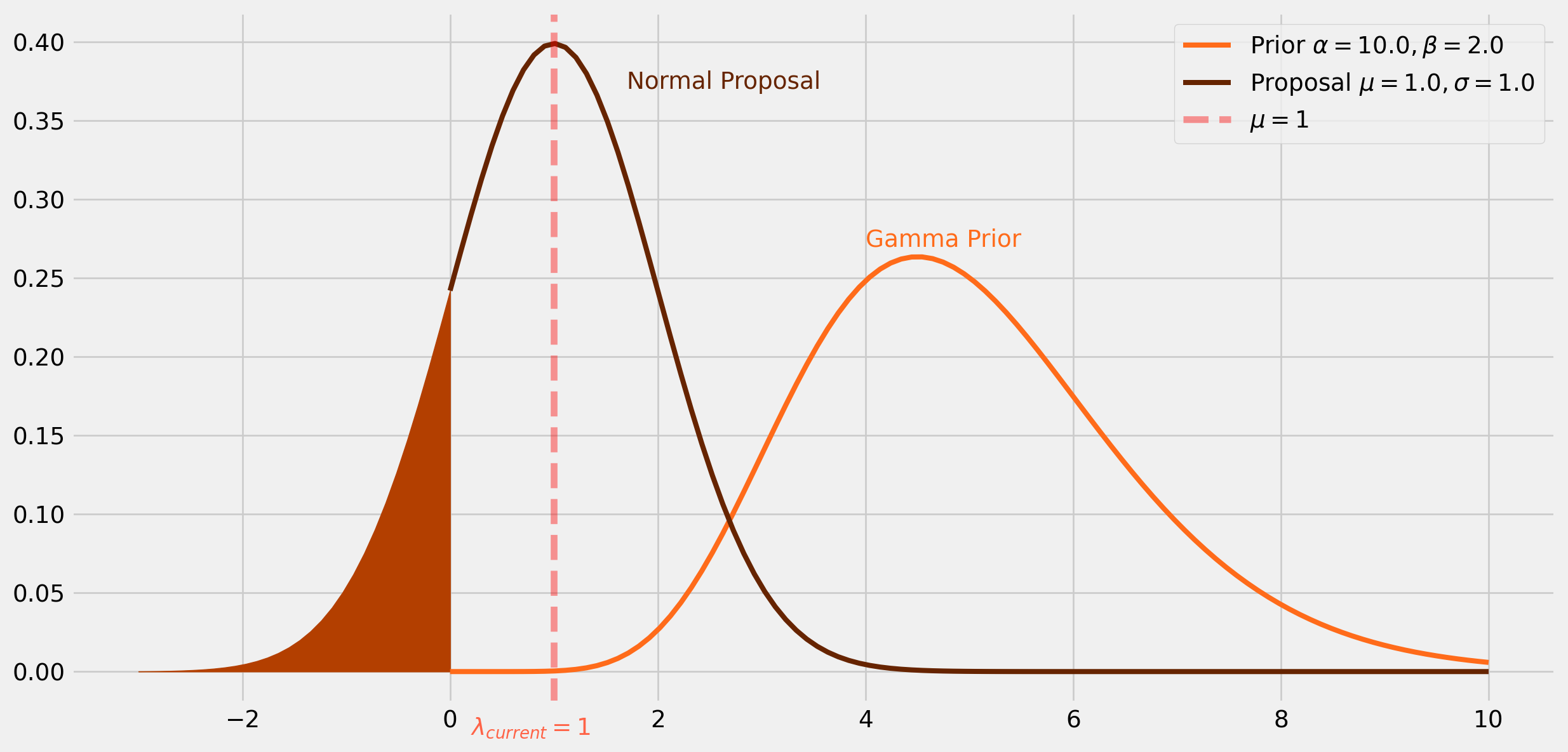
Two lines of codes will solve this issue
        if lamda_proposal < 0:
            lamda_proposal *= -1
def gamma_poisson_mcmc_1(
lamda_init=2, k=3, alpha=10, beta=2, tuning_param=1, chain_size=10000
):
np.random.seed(123)
lamda_current = lamda_init
lamda_mcmc = []
pass_rate = []
post_ratio_list = []
for i in range(chain_size):
lh_current = pois_lh(k=k, lamda=lamda_current)
prior_current = gamma_prior(alpha=alpha, beta=beta, lamda=lamda_current)
posterior_current = lh_current * prior_current
lamda_proposal = sp.stats.norm(loc=lamda_current, scale=tuning_param).rvs()
if lamda_proposal < 0:
lamda_proposal *= -1
prior_next = gamma_prior(alpha=alpha, beta=beta, lamda=lamda_proposal)
lh_next = pois_lh(k, lamda=lamda_proposal)
posterior_proposal = lh_next * prior_next
post_ratio = posterior_proposal / posterior_current
prob_next = np.min([post_ratio, 1])
unif_draw = sp.stats.uniform.rvs()
post_ratio_list.append(post_ratio)
if unif_draw < prob_next:
lamda_current = lamda_proposal
lamda_mcmc.append(lamda_current)
pass_rate.append("Y")
else:
lamda_mcmc.append(lamda_current)
pass_rate.append("N")
return lamda_mcmc, pass_rateThis time we can set chain size much larger.
lamda_mcmc, pass_rate = gamma_poisson_mcmc_1(chain_size=100000, tuning_param=1)As you can see the frequency distribution is also much smoother.
y_rate = pass_rate.count("Y") / len(pass_rate)
n_rate = pass_rate.count("N") / len(pass_rate)
yes = ["Pass", "Not Pass"]
counts = [pass_rate.count("Y"), pass_rate.count("N")]

fig, ax = plt.subplots(figsize=(12, 12), nrows=3, ncols=1)
ax[0].hist(lamda_mcmc[int(len(lamda_mcmc) / 10) :: 2], bins=100, density=True)
ax[0].set_title(r"Posterior Frequency Distribution of $\lambda$")
ax[0].plot(x, gamma_pdf_prior, label="Prior")
ax[0].plot(x, gamma_pdf_post, label="Posterior")
ax[0].legend()
ax[1].plot(np.arange(len(lamda_mcmc)), lamda_mcmc, lw=1)
ax[1].set_title("Trace")

ax[2].barh(yes, counts, color=["green", "blue"], alpha=0.7)
ax[2].text(
    counts[1] * 0.4,
    "Not Pass",
    r"${}\%$".format(np.round(n_rate * 100, 2)),
    color="tomato",
    size=28,
)
ax[2].text(
    counts[0] * 0.4,
    "Pass",
    r"${}\%$".format(np.round(y_rate * 100, 2)),
    color="tomato",
    size=28,
)
plt.show()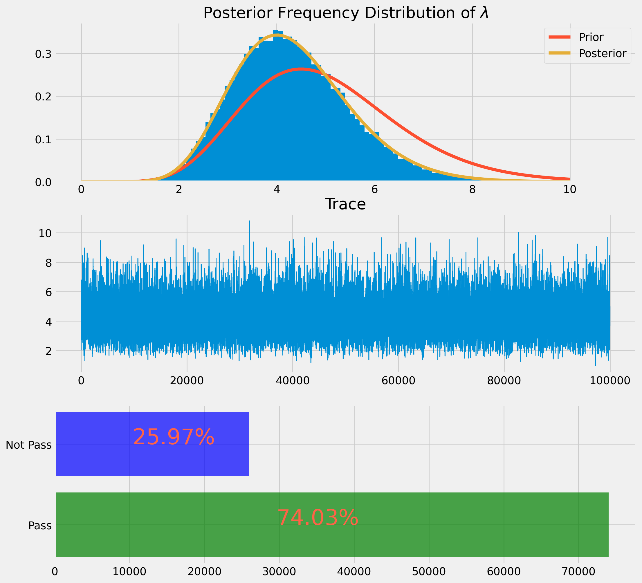
Numerical Overflow
If prior and likelihood are extremely close to \(0\), the product would be even closer to \(0\). This would cause storage error in computer due to the binary system.
The remedy is to use the log version of Bayes’ Theorem, i.e.
\[ \ln{P(\lambda \mid y)} \propto \ln{P(y \mid \lambda)}+ \ln{P(\lambda)} \]
Also the acceptance rule can be converted into log version
\[ \ln{ \left(\frac{P\left(\lambda_{proposed } \mid y \right)}{P\left(\lambda_{current} \mid y \right)}\right)} =\ln{P\left(\lambda_{proposed } \mid y \right)} - \ln{P\left(\lambda_{current } \mid y \right)} \]
def gamma_poisson_mcmc_2(
    lamda_init=2, k=3, alpha=10, beta=2, tuning_param=1, chain_size=10000
):
    np.random.seed(123)
    lamda_current = lamda_init

    lamda_mcmc = []
    pass_rate = []
    post_ratio_list = []

    for i in range(chain_size):
        log_lh_current = np.log(pois_lh(k=k, lamda=lamda_current))
        log_prior_current = np.log(
            gamma_prior(alpha=alpha, beta=beta, lamda=lamda_current)
        )
        log_posterior_current = log_lh_current + log_prior_current

        lamda_proposal = sp.stats.norm(loc=lamda_current, scale=tuning_param).rvs()
        if lamda_proposal < 0:
            lamda_proposal *= -1
        log_prior_next = np.log(
            gamma_prior(alpha=alpha, beta=beta, lamda=lamda_proposal)
        )
        log_lh_next = np.log(pois_lh(k, lamda=lamda_proposal))

        log_posterior_proposal = log_lh_next + log_prior_next
        log_post_ratio = log_posterior_proposal - log_posterior_current
        post_ratio = np.exp(log_post_ratio)

        prob_next = np.min([post_ratio, 1])
        unif_draw = sp.stats.uniform.rvs()
        post_ratio_list.append(post_ratio)

        if unif_draw < prob_next:
            lamda_current = lamda_proposal
            lamda_mcmc.append(lamda_current)
            pass_rate.append("Y")
        else:
            lamda_mcmc.append(lamda_current)
            pass_rate.append("N")
    return lamda_mcmc, pass_rate
With the use of log posterior and acceptance rule, the numerical overflow is unlikely to happen anymore, which means we can set a much longer Markov chain and also a larger tuning parameter.
lamda_mcmc, pass_rate = gamma_poisson_mcmc_2(chain_size=1000, tuning_param=3)y_rate = pass_rate.count("Y") / len(pass_rate)
n_rate = pass_rate.count("N") / len(pass_rate)
yes = ["Pass", "Not Pass"]
counts = [pass_rate.count("Y"), pass_rate.count("N")]
fig, ax = plt.subplots(figsize=(12, 12), nrows=3, ncols=1)
ax[0].hist(lamda_mcmc[int(len(lamda_mcmc) / 10) :: 2], bins=100, density=True)
ax[0].set_title(r"Posterior Frequency Distribution of $\lambda$")
ax[0].plot(x, gamma_pdf_prior, label="Prior")
ax[0].plot(x, gamma_pdf_post, label="Posterior")
ax[0].legend()
ax[1].plot(np.arange(len(lamda_mcmc)), lamda_mcmc, lw=1)
ax[1].set_title("Trace")
ax[2].barh(yes, counts, color=["green", "blue"], alpha=0.7)
ax[2].text(
counts[1] * 0.4,
"Not Pass",
r"${}\%$".format(np.round(n_rate * 100, 2)),
color="tomato",
size=28,
)
ax[2].text(
counts[0] * 0.4,
"Pass",
r"${}\%$".format(np.round(y_rate * 100, 2)),
color="tomato",
size=28,
)
plt.show()
Larger tuning parameter yields a lower pass (\(30\%\sim50\%\)) rate that is exactly what we are seeking for.
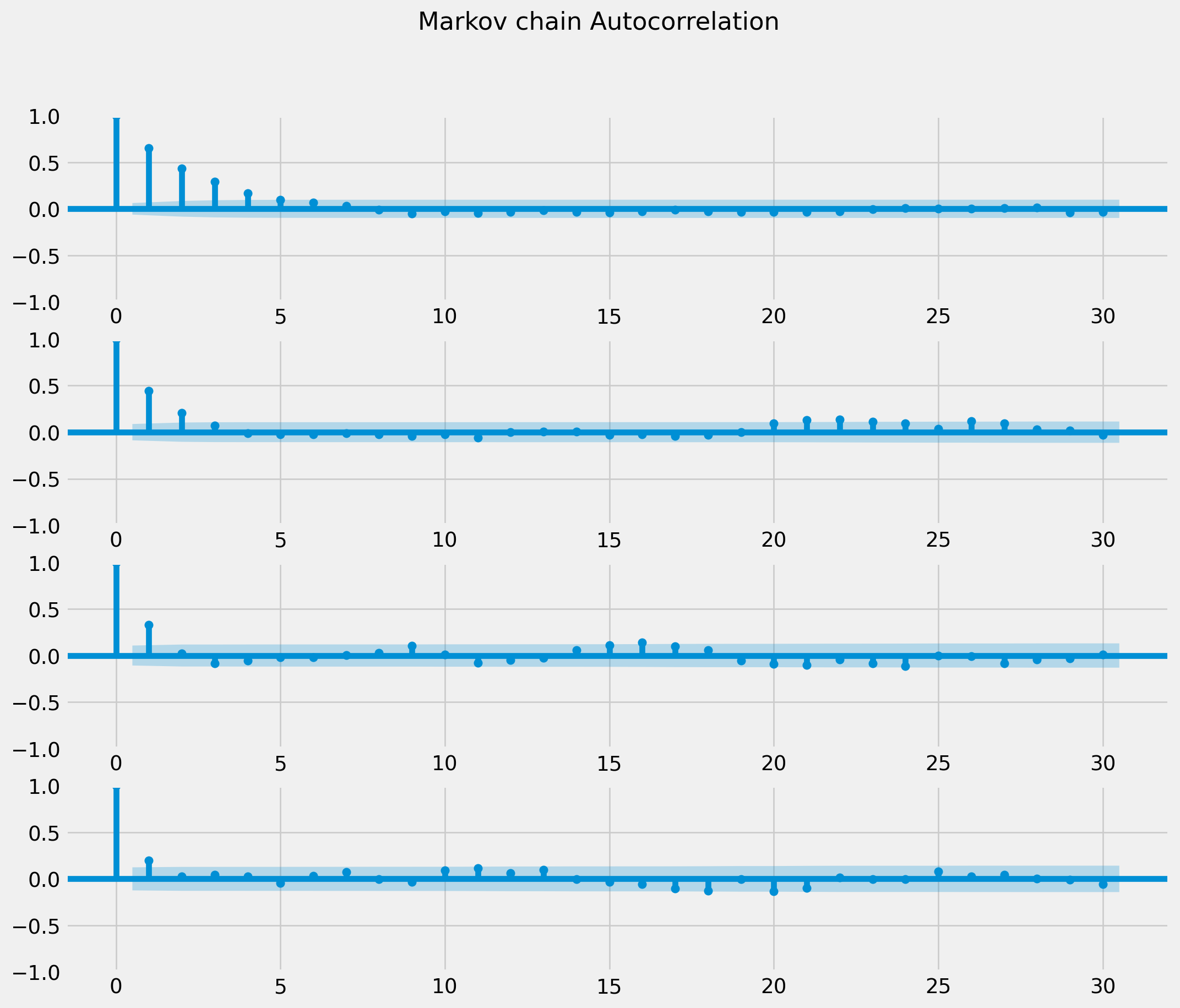
Pruning
lamda_mcmc = np.array(lamda_mcmc)
n = 4
fig, ax = plt.subplots(ncols=1, nrows=n, figsize=(12, 10))
for i in range(1, n + 1):
    g = plot_acf(
        lamda_mcmc[::i], ax=ax[i - 1], title="", label=r"$lag={}$".format(i), lags=30
    )
fig.suptitle("Markov chain Autocorrelation")

plt.show()